OpenCascade B-Spline Basis Function-卡核

OpenCascade B-Spline Basis Function

Abstract. B-splines are quite a bit more flexible than Bezier curves. This flexibility comes from the fact that you have much more control over the basis functions. For Bezier curves that each control point had an effect on each point on the curve; likewise the number of control points affected the degree of the curve. For the sake of flexiblity, you would like to be able to arbitrarily set the degree of the curve and to also determine the range of the affect each control point has. B-splines allow this level of control, the secret is its basis function. This paper focus on the B-splines basis function and some important properties of B-spline basis function, such as local support property, the multiplicity of the knot vector .etc.

Key words. B-spline Basis Function, OpenCascade B-spline, Multiplicity,

1. Introduction

在当前的CAD/CAM系统中，B样条曲线曲面已经成为几何造型系统的核心部分。B样条曲线曲面造型方法的理论基础就是B样条。Bezier曲线是以Bernstein基函数为基础的，虽然它有许多优点，但也有一些不足之处：

v 当给定了Bezier曲线的控制点后，也就确定了曲线的次数。当次数过高时，会给Bezier曲线的计算带来不便。如果采用分段三次Bezier曲线且要保持曲线间的连续性还必须有附加条件；

v Bezier曲线是整体定义的，改变任意一个控制点，将对整条曲线都有影响。因此Bezier不具有局部修改性。

1964年由Schoenberg提出了B样条理论，1972年de Boor与Cox分别独立给出了关于B样条的标准算法。Gordon和Riesenfeld又把B样条理论应用于形状描述，最终提出了B样条方法。用B样条代替Bernstein基，构造出B样条曲线，这种方法继承了Bezier方法的一切优点，克服了Bezier方法的缺点，较成功地解决了局部控制问题，又轻而易举地在参数连续性基础上解决了连接问题，从而使自由曲线曲面形状的描述问题得到较好解决。

B样条方法具有表示与设计自由曲线曲面的强大功能，它不仅是最广为流行的形状数学描述的主流方法之一，而且已成为关于工业产品几何定义国际标准的有理B样条方法的基础。从B样条理论的发展历程可以看出，理论与实践的相互作用。正是由于实际的需要，才提出解决问题的新方法。

本文给出B样条的递推定义并使用OpenCascade的B样条库在OpenSceneGraph中绘制出B样条基函数的曲线，在此基础上来理解B样条基函数的局部支撑性、节点向量的重复度等概念。

2. Definition of B-spline Basis Functions

有很多方法可以用来定义B样条基函数以及证明它的一些重要性质。例如可以采用截尾幂函数的差商定义，开花定义及由de Boor和Cox等人提出的递推公式等来定义。我们这里采用的是递推定义方法，因为这种方法在计算机实现中是最有效的。

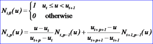
令U={u0,u1,…,um}是一个单调不减的实数序列，即ui<=ui+1，i=0,1,…,m-1。其中，ui称为节点，U称为节点矢量，用Ni,p(u)表示第i个p次B样条基函数，其定义为：

递推公式的几何意义可以归结为：移位、升阶和线性组合。由上述公式可知：

1) 当p>0时，Ni,p(u)是两个p-1次基函数的线性组合；

2) 计算一组基函数时需要事先指定节点矢量U和次数p；

3) 计算p次基函数的过程生成一个如下形式的三角阵列：

B样条基有如下性质：

a) 递推性；

b) 局部支承性；

c) 规范性；

d) 可微性；

关于B样条基函数更多的定义方式，可以参考《计算几何教程》、《自由曲线曲面造型技术》等。

3. Use OpenCascade B-spline Library

在OpenCascade中，B样条的计算库位于基础模块（FoundationClasses Module）的TKMath，有分别对曲线和曲面的底层计算类BSplCLib和BSplSLib。关于B样条曲线计算库中对B样条基函数计算的实现方法见：B-Spline Curve Library in Open Cascade

http://www.cppblog.com/eryar/archive/2013/03/12/198367.html 。本文主要介绍将B样条基函数的计算结果在OpenSceneGraph中显示出来，以便于直观的理解B样条基的相关性质。程序代码如下所示：

/*
*    Copyright (c) 2014 eryar All Rights Reserved.
*
*        File    : Main.cpp
*        Author  : eryar@163.com
*        Date    : 2014-07-20 20:46
*        Version : 1.0v
*
*    Description : Show OpenCascade B-Spline Basis evaluate 
*                  result in OpenSceneGraph.
*
*      Key words : OpenCascade, OpenSceneGraph, 
*                  B-Spline Basis Function
*/

// OpenSceneGraph library.
#include <osg/MatrixTransform>

#include <osgDB/ReadFile>
#include <osgViewer/Viewer>
#include <osgGA/StateSetManipulator>
#include <osgViewer/ViewerEventHandlers>

#pragma comment(lib, \"osgd.lib\")
#pragma comment(lib, \"osgDBd.lib\")
#pragma comment(lib, \"osgGAd.lib\")
#pragma comment(lib, \"osgViewerd.lib\")

// OpenCASCADE library.
#define WNT

#include <TColStd_Array1OfReal.hxx>
#include <math_Matrix.hxx>
#include <BSplCLib.hxx>

#pragma comment(lib, \"TKernel.lib\")
#pragma comment(lib, \"TKMath.lib\")

osg::Node* BuildAxes(Standard_Real x, Standard_Real y)
{
    osg::ref_ptr<osg::Geode> aGeode = new osg::Geode();
    osg::ref_ptr<osg::Geometry> aLineGeom = new osg::Geometry();
    osg::ref_ptr<osg::Vec3Array> aVertices = new osg::Vec3Array();

    // x axis
    aVertices->push_back(osg::Vec3(0.0, 0.0, 0.0));
    aVertices->push_back(osg::Vec3(x + 0.5, 0.0, 0.0));

    // arrow for x axis
    aVertices->push_back(osg::Vec3(x + 0.5, 0.0, 0.0));
    aVertices->push_back(osg::Vec3(x + 0.3, 0.0, 0.05));

    aVertices->push_back(osg::Vec3(x + 0.5, 0.0, 0.0));
    aVertices->push_back(osg::Vec3(x + 0.3, 0.0, -0.05));

    // x ruler
    for (Standard_Integer i = 1; i <= x; ++i)
    {
        aVertices->push_back(osg::Vec3(i, 0.0, 0.05));
        aVertices->push_back(osg::Vec3(i, 0.0, -0.05));
    }

    // y axis
    aVertices->push_back(osg::Vec3(0.0, 0.0, 0.0));
    aVertices->push_back(osg::Vec3(0.0, 0.0, y + 0.5));

    // arrow for y axis
    aVertices->push_back(osg::Vec3(0.0, 0.0, y + 0.5));
    aVertices->push_back(osg::Vec3(0.05, 0.0, y + 0.3));

    aVertices->push_back(osg::Vec3(0.0, 0.0, y + 0.5));
    aVertices->push_back(osg::Vec3(-0.05, 0.0, y + 0.3));

    // y ruler
    for (Standard_Integer j = 1; j <= y; ++j)
    {
        aVertices->push_back(osg::Vec3(0.05, 0.0, j));
        aVertices->push_back(osg::Vec3(-0.05, 0.0, j));
    }

    aLineGeom->setVertexArray(aVertices);
    aLineGeom->addPrimitiveSet(new osg::DrawArrays(osg::PrimitiveSet::LINES, 0, aVertices->size()));

    aGeode->addDrawable(aLineGeom);
    return aGeode.release();
}

osg::Node* BuildBSplineBasis(const TColStd_Array1OfReal &theKnots, int theDegree)
{
    osg::ref_ptr<osg::Group> aGroup = new osg::Group();
    osg::ref_ptr<osg::Geode> aGeode = new osg::Geode();
    osg::ref_ptr<osg::Geometry> aPointGeom = new osg::Geometry();
    osg::ref_ptr<osg::Vec3Array> aVertices = new osg::Vec3Array();

    Standard_Integer aIndex = 0;
    Standard_Integer aOrder = theDegree + 1;
    math_Matrix m(1, 1, 1, aOrder);

    for (Standard_Real u = theKnots.Value(theKnots.Lower()); u <= theKnots.Value(theKnots.Upper()); u += 0.001)
    {
        BSplCLib::EvalBsplineBasis(0, 0, aOrder, theKnots, u, aIndex, m);

        for (Standard_Integer i = 1; i <= aOrder; ++i)
        {
            aVertices->push_back(osg::Vec3(u, 0.0, m(1, i)));
        }
    }

    aPointGeom->setVertexArray(aVertices);
    aPointGeom->addPrimitiveSet(new osg::DrawArrays(osg::PrimitiveSet::POINTS, 0, aVertices->size()));

    // set the color for the points.
    osg::ref_ptr<osg::Vec4Array> aColor = new osg::Vec4Array();
    aColor->push_back(osg::Vec4(aOrder % 1, aOrder % 2, aOrder % 3, 1.0));

    aPointGeom->setColorArray(aColor);
    aPointGeom->setColorBinding(osg::Geometry::BIND_OVERALL);

    aGeode->addDrawable(aPointGeom);

    aGroup->addChild(aGeode);
    aGroup->addChild(BuildAxes(theKnots.Value(theKnots.Upper()), 1.0));

    return aGroup.release();
}

osg::Node* BuildBSplineBasis(void)
{
    osg::ref_ptr<osg::Group> aGroupNode = new osg::Group();
    TColStd_Array1OfReal aKnots1(1, 8);

    aKnots1(1) = 0.0;
    aKnots1(2) = 0.0;
    aKnots1(3) = 0.0;
    aKnots1(4) = 0.0;
    aKnots1(5) = 1.0;
    aKnots1(6) = 1.0;
    aKnots1(7) = 1.0;
    aKnots1(8) = 1.0;

    osg::ref_ptr<osg::MatrixTransform> aUniformBasis = new osg::MatrixTransform();
    aUniformBasis->setMatrix(osg::Matrix::translate(0.0, 0.0, 0.0));
    aUniformBasis->addChild(BuildBSplineBasis(aKnots1, 4));

    aGroupNode->addChild(aUniformBasis);
    return aGroupNode.release();
}

int main(int argc, char* argv[])
{
    osgViewer::Viewer aViewer;

    aViewer.setSceneData(BuildBSplineBasis());

    aViewer.addEventHandler(new osgGA::StateSetManipulator(aViewer.getCamera()->getOrCreateStateSet()));
    aViewer.addEventHandler(new osgViewer::StatsHandler);
    aViewer.addEventHandler(new osgViewer::WindowSizeHandler);

    return aViewer.run();
}

B样条基函数计算使用了函数BSplCLib::EvalBsplineBasis()，通过这个函数不仅可以计算基函数，还可以计算B样条基函数的导数。计算结果输出到一个矩阵之中。根据定义可知要计算B样条基函数，需要指定节点矢量和次数，所以函数BuildBSplineBasis()就根据这两个参数生成B样条基函数的图形进行显示。上述代码生成的一个B样条基函数结果如下图所示：

Figure 3.1 U=[0,0,0,0,1,1,1,1], p=4的B样条基函数

改变次数，生成p=3时的基函数如下图所示：

Figure 3.2 U=[0,0,0,0,1,1,1,1], p=3的B样条基函数

4. Local Support Property

B样条的局部支承性（Local Support Property）是B样条最重要的性质之一，也是B样条方法与Bezier方法的主要差别所在。由于局部支承性质，使B样条曲线具有良好的局部性，从而为曲线、曲面设计奠定了良好的基础。

Figure 4.1 Local Support Property of B-spline Basis Function

从上图可以看出，N1,3是N1,0，N2,0，N3,0，N4,0的线性组合，所以N1,3的非零区域只在u∈[u1, u5]，即：

上式表明，第i条k次B样条仅在节点ti到ti+k+1的k+1个区间内不为0，其他区间均为0.这个性质称为局部支承性。

k次B样条仅在k+1个区间内非0。换言之，每段k次B样条曲线只涉及k+1个基函数，并由k+1个顶点所定义。B样条的局部支承性对曲线、曲面设计有两方面的影响：

v 第i段k次B样条曲线仅由Pi, Pi+1, …, Pi+k共k+1个顶点所控制，而与其他顶点无关。为此，为修改一段曲线，仅需修改有关的k+1个顶点即可；

v 反之，修改一个顶点，对B样条曲线的影响也是局部的，对于均匀的k次B样条曲线调整一个顶点的位置仅影响与该顶点有关的k+1段曲线。

局部支承性是B样条方法最引人的特点之一。

5. Multiplicity of the Knot Vector

重节点连续阶性质：在每一个节点区间(ui, ui+1)内部，Ni,p(u)为多项式，因此有导数存在。在一个节点ui处，Ni,p(u)是一个p-mi次连续可微的，此处mi是该节点的重数（Multiplicity）。所以增加次数，则增加连续性，而增加节点的重数，则降低连续性。

节点矢量U={0, 0, 0, 1, 2, 3, 4, 4, 5, 5, 5}上的2次B样条基函数如下图所示：

Figure 5.1 U={0, 0, 0, 1, 2, 3, 4, 4, 5, 5, 5} p = 2 B-spline Basis Function

程序代码如下所示：

TColStd_Array1OfReal aKnots2(1, 11);

aKnots2(1) = 0.0;
aKnots2(2) = 0.0;
aKnots2(3) = 0.0;
aKnots2(4) = 1.0;
aKnots2(5) = 2.0;
aKnots2(6) = 3.0;
aKnots2(7) = 4.0;
aKnots2(8) = 4.0;
aKnots2(9) = 5.0;
aKnots2(10) = 5.0;
aKnots2(11) = 5.0;

osg::ref_ptr<osg::MatrixTransform> aNonUniformBasis2 = new osg::MatrixTransform();
aNonUniformBasis2->addChild(BuildBSplineBasis(aKnots2, 2));
aGroupNode->addChild(aNonUniformBasis2);

从上图可知，在节点u=4的位置，B样条基函数的曲线已经失去了连续性。再举一个例子，节点矢量U＝{0,0,0,0,1,2,3,4,4,4,5,5,5,5}，p=3的B样条基函数如下图所示：

Figure 5.2 U={0, 0, 0, 0,1, 2, 3, 4, 4,4, 5, 5, 5,5} p = 3 B-spline Basis Function

当节点矢量两端的重复度如下所示时，则B样条基函数退化为Bernstein基函数：

因此，Bezier可以看作是B样条表达式的一种特例。在OpenCascade的B样条计算类中有一个函数可以根据次数p来生成Bezier的节点矢量：

//=====================================================================
// function: FlatBezierKnots
// purpose :
//=====================================================================
// array of flat knots for bezier curve of maximum 25 degree
static const Standard_Real knots[52] = { 0, 0, 0, 0, 0, 0, 0, 0, 0, 0, 0, 0, 0, 0, 0, 0, 0, 0, 0, 0, 0, 0, 0, 0, 0, 0, 
                                         1, 1, 1, 1, 1, 1, 1, 1, 1, 1, 1, 1, 1, 1, 1, 1, 1, 1, 1, 1, 1, 1, 1, 1, 1, 1 };
const Standard_Real& BSplCLib::FlatBezierKnots (const Standard_Integer Degree)
{
  Standard_OutOfRange_Raise_if (Degree < 1 || Degree > MaxDegree() || MaxDegree() != 25,
    \"Bezier curve degree greater than maximal supported\");

  return knots[25-Degree];
}