最小二乘法拟合直线

在科学实验和生产实践中，经常需要从一组实验数据出发寻求函数y=f(x)的一个近似表达式，也称为经验公式。从几何上看，就是希望根据给定的m个点，求曲线y=f(x)的一条近似曲线。因此这是个曲线拟合问题。

当我们要求近似曲线严格通过给定的每个点时，这是插值算法。对于本文所述的直线拟合来说，如果用插值算法，则只需要两个点就够了。实际直线拟合数据可能满足不了这个条件，为了便于计算，分析与应用，我们较多地根据“使测量点到直线距离的平方和最小”的原则来拟合。按最小二乘原则选择拟合曲线的方法，称为最小二乘法（Method of Least Squares）。

利用最小二乘法拟合曲线的一般步骤是：

将实验数据显示出来，分析曲线的形式；
确定拟合曲线的形式。对于本文来说，曲线形式是直线，y=a+bx;
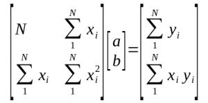
建立法方程组并对其进行求解；

因为OpenCASCADE中数据结构及算法丰富，所以用OpenCASCADE可以快速实现直线的最小二乘法拟合算法。下面给出具体实现代码：

#include <iostream>

#include <gp_Lin2d.hxx>
#include <gp_Pnt2d.hxx>

#include <TColgp_Array1OfPnt2d.hxx>

#include <math_Vector.hxx>
#include <math_SVD.hxx>
#include <math_Gauss.hxx>
#include <math_GaussLeastSquare.hxx>

#include <OSD_Chronometer.hxx>


void fitLine(const TColgp_Array1OfPnt2d& thePoints,
             const std::string& theFileName,
             gp_Lin2d& theLine)
{
    math_Vector aB(1, 2, 0.0);
    math_Vector aX(1, 2, 0.0);
    math_Matrix aM(1, 2, 1, 2);

    Standard_Real aSxi = 0.0;
    Standard_Real aSyi = 0.0;
    Standard_Real aSxx = 0.0;
    Standard_Real aSxy = 0.0;

    std::ofstream aDrawFile(theFileName);

    for (Standard_Integer i = thePoints.Lower(); i <= thePoints.Upper(); ++i)
    {
        const gp_Pnt2d& aPoint = thePoints.Value(i);

        aSxi += aPoint.X();
        aSyi += aPoint.Y();

        aSxx += aPoint.X() * aPoint.X();
        aSxy += aPoint.X() * aPoint.Y();

        aDrawFile << \"vpoint p\" << i << \" \" <<
                     aPoint.X() << \" \" << aPoint.Y() << \" 0\" << std::endl;
    }

    aM(1, 1) = thePoints.Size();
    aM(1, 2) = aSxi;
    aM(2, 1) = aSxi;
    aM(2, 2) = aSxx;

    aB(1) = aSyi;
    aB(2) = aSxy;

    OSD_Chronometer aChronometer;
    aChronometer.Start();

    math_Gauss aSolver(aM);
    //math_GaussLeastSquare aSolver(aM);
    //math_SVD aSolver(aM);
    aSolver.Solve(aB, aX);
    if (aSolver.IsDone())
    {
        Standard_Real aA = aX(1);
        Standard_Real aB = aX(2);

        gp_Pnt2d aP1(0.0, aA);
        gp_Pnt2d aP2(-aA/aB, 0.0);

        theLine.SetLocation(aP1);
        theLine.SetDirection(gp_Vec2d(aP1, aP2).XY());

        aDrawFile << \"vaxis l \"
                  << aP1.X() << \" \" << aP1.Y() << \" 0 \"
                  << aP2.X() << \" \" << aP2.Y() << \" 0 \" << std::endl;

        std::cout << \"===================\" << std::endl;
        aX.Dump(std::cout);
    }

    aChronometer.Stop();
    aChronometer.Show();
}

int main()
{
    gp_Lin2d aLine;

    // Test data 1
    TColgp_Array1OfPnt2d aPoints1(1, 6);
    aPoints1.SetValue(1, gp_Pnt2d(36.9, 181.0));
    aPoints1.SetValue(2, gp_Pnt2d(46.7, 197.0));
    aPoints1.SetValue(3, gp_Pnt2d(63.7, 235.0));
    aPoints1.SetValue(4, gp_Pnt2d(77.8, 270.0));
    aPoints1.SetValue(5, gp_Pnt2d(84.0, 283.0));
    aPoints1.SetValue(6, gp_Pnt2d(87.5, 292.0));

    fitLine(aPoints1, \"fit1.tcl\", aLine);

    // Test data 2
    TColgp_Array1OfPnt2d aPoints2(0, 7);
    aPoints2.SetValue(0, gp_Pnt2d(0.0, 27.0));
    aPoints2.SetValue(1, gp_Pnt2d(1.0, 26.8));
    aPoints2.SetValue(2, gp_Pnt2d(2.0, 26.5));
    aPoints2.SetValue(3, gp_Pnt2d(3.0, 26.3));
    aPoints2.SetValue(4, gp_Pnt2d(4.0, 26.1));
    aPoints2.SetValue(5, gp_Pnt2d(5.0, 25.7));
    aPoints2.SetValue(6, gp_Pnt2d(6.0, 25.3));
    aPoints2.SetValue(7, gp_Pnt2d(7.0, 24.8));

    fitLine(aPoints2, \"fit2.tcl\", aLine);

    return 0;
}

在函数fitLine()中，根据拟合点建立法方程组，并使用math_Gauss来对法方程组进行求解。其实也可以使用math_GaussLeastSquare或者math_SVD等求解法方程组。在主函数main()中测试了两组数据。测试数据1来自易大义等《计算方法》，测试数据2来自《高等数学》。程序运行结果如下图所示：

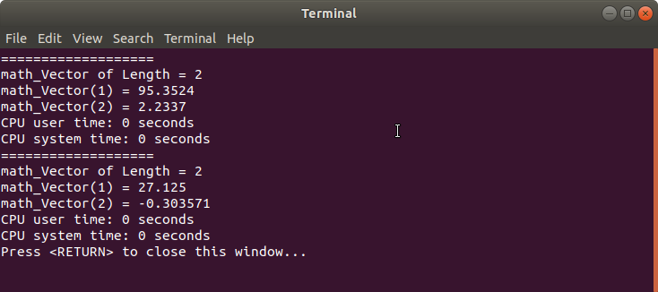
与书中计算结果吻合。

由于需要将计算结果显示出来，所以在fitLine()函数中增加了输出Draw脚本文件的代码，实际运用时可将这部分代码去掉。将程序生成的脚本文件加载到Draw中，即可得到下面两个图：

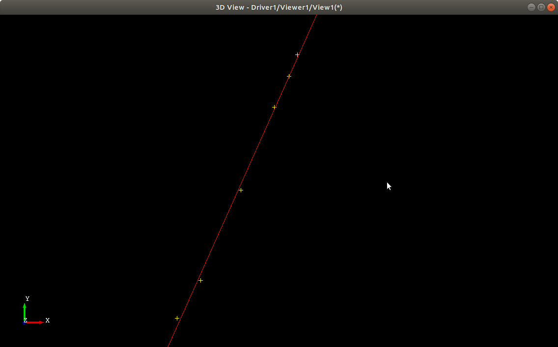
测试数据1拟合直线

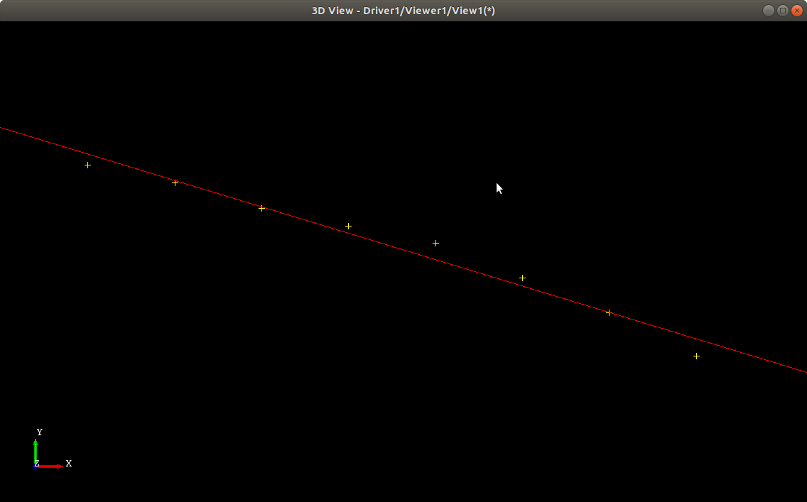
测试数据2拟合直线

综上所述，对于二维直线的最小二乘法拟合算法的关键是对建立的法方程组进行求解。OpenCASCADE的math包中提供了一些解方程组的类可以直接使用。对于没有使用OpenCASCADE的开发环境的情况，也可以使用其他矩阵库，如Eigen等用得很广泛。Eigen官方网站：http://eigen.tuxfamily.org/index.php?title=Main_Page

将计算结果导出Draw脚本可视化，可以方便直观地查看拟合结果。如果熟悉其他脚本库如Python的matplotlib，也可以类似处理来将结果可视化。

pre { direction: ltr; color: rgba(0, 0, 0, 1); text-align: left }
pre.western { }
pre.cjk { font-family: \”DejaVu Sans Mono\”, monospace }
pre.ctl { }
h1 { margin-bottom: 0.21cm; direction: ltr; color: rgba(0, 0, 0, 1); text-align: left }
h1.western { font-family: \”Liberation Sans\”, serif; font-size: 18pt }
h1.cjk { font-family: \”Noto Sans CJK SC Regular\”; font-size: 18pt }
h1.ctl { font-family: \”Lohit Devanagari\”; font-size: 18pt }
p { margin-bottom: 0.25cm; direction: ltr; color: rgba(0, 0, 0, 1); line-height: 115%; text-align: left }
p.western { }
p.cjk { }
p.ctl { }
a:link { }

文章版权归作者所有，未经允许请勿转载。

THE END

OCC源码学习几何造型器
# opencascade code study